The standard model
Before explaining how an overclock is calculated, it helps to review how times are calculated in a standard model — one involving under-speed, or a longer loss.
With each pulse collected, the system classifies the theoretical duration for producing a part as normal time: the theoretical cycle time, shown in green on the diagram.
If the actual production time of a part exceeds its theoretical cycle time, the excess is recorded as a loss, shown in red.
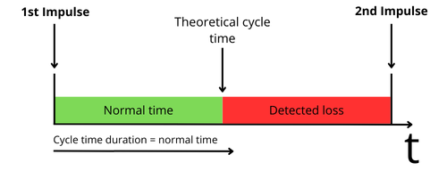
The green duration (normal time) and the red one (the detected loss) are both consumed between the two pulses. To avoid recording a loss, the theoretical cycle time of a part must be strictly respected.
The overclock case
When an overclock is detected — because the machine is faster than expected — the situation is the opposite. The system detects a loss not because the theoretical cycle time has been exceeded, but because it has never been reached.
When a pulse is recorded by the module before the end of the theoretical cycle time configured for a given product, the tablet records an overclock.
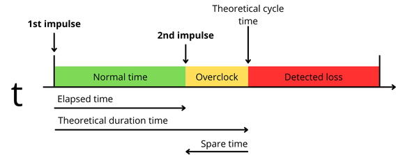
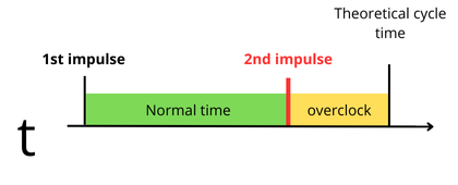
On the diagram above, a pulse 1 is recorded, marking the start of the production of a part. A pulse 2 appears before the theoretical cycle time is over, which triggers an overclock.
That overclock is automatically informed under the loss type you configured on the platform, in PerfTrak > Loss Configurations > Configuration.
The formula
(Time between pulse 1 and pulse 2) − Theoretical cycle time = Displayed loss duration
The same formula applies in the classic case, where the cycle time is exceeded, and in the opposite case, where the production time is shorter than the cycle time — the overclock case.
Example. For a product with a cycle time of 10 seconds, with a pulse 2 recorded 8 seconds after pulse 1:
8 − 10 = −2 seconds
The duration obtained is negative, since the production time is shorter than the cycle time: the machine is running faster than the pace set by the theoretical cycle time.